In order to make a image classification problem, I decided to make a little experiment, comparing two different Neural Network arquictectures, PyTorch and Tensorflow (using Keras).

PyTorch is an open source machine learning library primarily developed by Facebook’s AI Research lab (FAIR), whileTensorFlow was developed by the Google Brain team for internal Google use, although nowadays it is free to use for anybody. For a simpler management of TensorFlow, I use the Keras framework, which eases the complex grammar TF uses.

Data

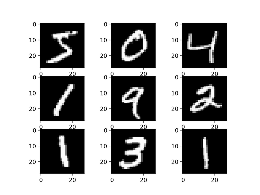
For this experiment, we will be using the ‘MNIST’ dataset. It is a really large dataset (70.000 samples) of handwritten digits. The training set contains 60.000 samples, white the testing set has another 10.000 ones. This dataset is already integrated in most frameworks and it is quite extended. You can see an example of this dataset in the figure below.

TensorFlow

We will start with TensorFlow. We start loading the data

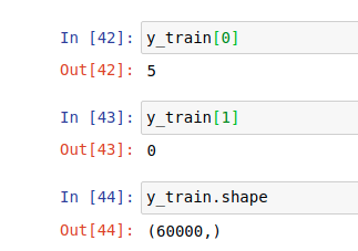
from keras import *(x_train, y_train), (x_test, y_test) = keras.datasets.mnist.load_data()

As said earlier, this dataset is included in the keras framework. Now, the shape of this loaded tensor is 60000 samples of 28×28, which makes a tridimensional tensor (60000, 28, 28). We may use a convolutional network, but doing it that way it would take a lot of time. Instead, we may convert this tensor to a (60000, 28*28) bidimensional tensor. Also, the data comes as 256 bit data, we are interested in normalizing this data, which we may do simply dividing by 255 (since it goes from 0 to 255).

#Normalizing data
x_train = x_train.astype("float32") / 255
x_test = x_test.astype("float32") / 255
# Reshaping (60000, 28, 28) into (60000, 28*28)
x_train = x_train.reshape(x_train.shape[0], x_train.shape[1]* x_train.shape[1])
x_test = x_test.reshape(x_test.shape[0], x_test.shape[1]*x_test.shape[1])

Now, we convert the ‘y’ part to categorical. Instead of having a single number represented (1, 2, 3…9) we have binary 10-shaped matrix, representing those single numbers using 0s and 1s.

num_classes = 10
y_train = keras.utils.to_categorical(y_train, num_classes)
y_test = keras.utils.to_categorical(y_test, num_classes)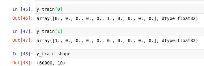

Now, as we were saying earlier we use a simple ‘Dense’ based neural network. For this experiment we test different activation functions, optimizers and layer combinations.

First, 3 different neural networks using a 3 layer neural network, using the following combination:

model1 = Sequential()
model1.add(Dense(128, activation=’linear’))
model1.add(Dense(64, activation=’relu’))
model1.add(Dense(10, activation=’softmax’))

For each of these we use a different optimizer. Usually, for many problems I use Adamax or RMSprop as optimizers, this time I add SGD. For the loss measure I use ‘categorical_crossentropy’ and for the metrics on testing I use ‘accuracy’.

model1.compile(optimizer=keras.optimizers.Adamax(lr=0.03), loss=’categorical_crossentropy’, metrics = [‘accuracy’])model2.compile(optimizer=keras.optimizers.RMSprop(lr=0.03), loss='categorical_crossentropy', metrics = ['accuracy'])model3.compile(optimizer=keras.optimizers.SGD(lr=0.03), loss='categorical_crossentropy', metrics = ['accuracy'])

Also, I try another combination of layers, adding a fourth layer, that would look like this

model61 = Sequential()
model61.add(Dense(256, activation='relu'))
model61.add(Dense(128, activation='linear'))
model61.add(Dense(64, activation='relu'))
model61.add(Dense(10, activation='softmax'))model61.compile(optimizer=keras.optimizers.SGD(lr=0.03), loss='categorical_crossentropy', metrics = ['accuracy'])

On the literature is recommended to use softmax or similar activation functions for classification problem, it is demonstrate during this exercise that softmax activations in the last layer end up getting us better results.

The best result overall would be the following:

model62 = Sequential()
model62.add(Dense(256, activation=’relu’))
model62.add(Dense(128, activation=’relu’))
model62.add(Dense(64, activation=’relu’))
model62.add(Dense(10, activation=’softmax’))
model62.compile(optimizer=keras.optimizers.SGD(lr=0.03), loss=’categorical_crossentropy’, metrics = [‘accuracy’])model62.fit(x_train, y_train, epochs=5, verbose=1, batch_size=20)
score = model62.evaluate(x_test, y_test, verbose=0)

This model obtained a 97.5% (0.077 cross-entropy) and 98% accuracy respectively on test and train phases. Training and testing this model lasted 1’45”, which is a pretty decent result, despite here we only iterate the model 5 times. Using 15 epochs instead of 5 we obtain a 99.8% accuracy on the training, but the testing accuracy only goes up to 98%, so it’s probably an innecessary overfitting.

PyTorch

Now, for PyTorch we kinda follow the same paths. First, we import the data (integrated in PyTorch framework as well). PyTorch is a bit different, since we have to create first a transformer to set the kind of data we want to have, and then get a trainloader and testloader (train=False/True).

# We import the data from 'datasets.MNIST', PyTorch allows us to directly normalize the data on the importation. To do that we setup a transformer that will create a normalized tensor ('transform').transform = transforms.Compose([transforms.ToTensor(),transforms.Normalize((0.5,), (0.5,)),])trainset = datasets.MNIST('~/.pytorch/MNIST_data/', download=True, train=True, transform=transform)trainloader = torch.utils.data.DataLoader(trainset, batch_size=20)testset = datasets.MNIST('~/.pytorch/MNIST_data/', download=True, train=False, transform=transform)testloader = torch.utils.data.DataLoader(testset, batch_size=20)

The dataloader utility from PyTorch allow us to differentiate between labels and data:

images, labels = next(iter(trainloader))

The images are loaded in iterations using the trainloader. Using the ‘view’ feature, we reshape the tensors into a bidimensional tensor.

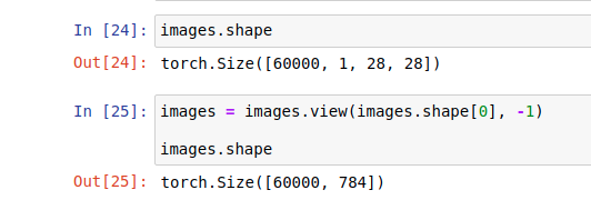
images = images.view(images.shape[0], -1)

Now, we have our data ready, we can create our model. The models created will have structures similar to the ones we used on Keras (activation functions, optimizers, layers…).

First, we define the layers of our model, which would be something like this (the numbers refer to the entering and the outgoing shapes).

model8 = nn.Sequential(nn.Linear(784, 256),
                      nn.ReLU(),
                      nn.Linear(256, 128),
                      nn.Softmax(),
                      nn.Linear(128, 64),
                      nn.ReLU(),
                      nn.Linear(64, 10))

Now, the loss criterion and the optimizer.

criterion = nn.CrossEntropyLoss()
optimizer = optim.Adamax(model8.parameters(), lr=0.003)

The model is set, we now have to train it and then test the results. We set 5 iterations, and make it run over the loader. We also gotta set ‘optimizer.zero_grad’ to make the weights reset and make the back-propagation run using ‘loss.backward’. The loss on the training set is stored on ‘running_loss’ which is printed after each iteration ending.

epochs = 5
for e in range(epochs):
    running_loss = 0
    for images, labels in trainloader:
        images = images.view(images.shape[0], -1)
    
        optimizer.zero_grad()
        
        output = model8(images)
        loss = criterion(output, labels)
        loss.backward()
        optimizer.step()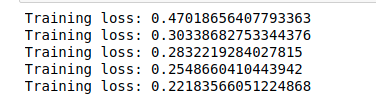

The best model obtained the cross-entropy error on the training phase of 0.10 (vs just 0.0479 obtained using Keras), so it seems like keras has outperformed its PyTorch counterpart. However, when we check out the accuracy reports (that we can obtain with the next piece of code), we see that PyTorch got an outstanding 100% accuracy on both training and test sets, vs the 98–97.5% on Keras using the same number of iterations and batch sizes.

top_p, top_class = output.topk(1, dim=1)equals = top_class == labels.view(*top_class.shape)
accuracy = torch.mean(equals.type(torch.FloatTensor))
print(f'Accuracy: {accuracy.item()*100}%')

We can see the PyTorch results on this little piece of code, which let us graphically check labels vs images .

%matplotlib inline
import helperimages, labels = next(iter(trainloader))img = images[0].view(1, 784)logps = model8(img)ps = torch.exp(logps)
helper.view_classify(img.view(1, 28, 28), ps)

If you want thenotebooks used on this little experimnt they are available to download from our git: https://github.com/ATG-Analytical/Image-Classification.git