Based on the approach of this article (Spanish): https://medium.com/atg-analytical/que-nos-deparar%C3%A1-el-coronavirus-548f3b87ebcd

In short, we are predicting the number of deaths in UK for the next 5 days based in 3 groups of factors:

• Propagation (20 and 15 days before the prediction)
• Total deaths (10 and 5 days before the prediction)
• Days since community propagation starts, counting day 0 = 10 days before the total number of deaths arrive to 5 (same day of the prediction)

This way we can predict at least 5 days, or even more if we add our predicted deaths to the data, but that would be a prediction based on other predictions, so for start we will simply do this 5 day prediction.

So, let’s start explaining the notebook. First of all, importing the basic libraries we’ll need later. These are just pandas, to shape our dataframes, bokeh, which is the library I use for graphic representation and some math modules.

import pandas as pd 
from bokeh.models import ColumnDataSource, Range1d, LabelSet, Label
from bokeh.plotting import figure, output_file, show
from bokeh.models import ColumnDataSource, Range1d, LabelSet, Label
from bokeh.plotting import figure, output_file, show
from bokeh.layouts import gridplot
import numpy as np
import math
import urllib
from numpy import inf

Our data is imported from the ECDC, and it allows downloading it from script, so we can keep updated the notebook.

link = ‘https://covid.ourworldindata.org/data/ecdc/full_data.csv'
urllib.request.urlretrieve(link, ‘Descargas/full_data.csv’)

Before getting into proper work, it is mandatory to do some data exploration. Here I create differente dataframes for the countries i want to have a look at, where I check their death, propagation, mortality rates, etc.

Data = pd.read_csv(‘Descargas/full_data.csv’).fillna(0)
SpainCases = Data[Data[‘location’]==’Spain’].drop(‘location’, axis=1)
ItalyCases = Data[Data[‘location’]==’Italy’].drop(‘location’, axis=1)
ChinaCases = Data[Data[‘location’]==’China’].drop(‘location’, axis=1)
GermanyCases = Data[Data[‘location’]==’Germany’].drop(‘location’, axis=1)
FranceCases = Data[Data[‘location’]==’France’].drop(‘location’, axis=1)
UKCases = Data[Data[‘location’]==’United Kingdom’].drop(‘location’, axis=1)
KoreaCases = Data[Data[‘location’]==’South Korea’].drop(‘location’, axis=1)
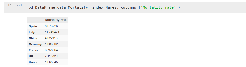
SpainMortality = SpainCases[‘total_deaths’][-1:]/SpainCases[‘total_cases’][-1:]*100
ItalyMortality = ItalyCases[‘total_deaths’][-1:]/ItalyCases[‘total_cases’][-1:]*100
ChinaMortality = ChinaCases[‘total_deaths’][-1:]/ChinaCases[‘total_cases’][-1:]*100
GermanyMortality = GermanyCases[‘total_deaths’][-1:]/GermanyCases[‘total_cases’][-1:]*100
FranceMortality = FranceCases[‘total_deaths’][-1:]/FranceCases[‘total_cases’][-1:]*100
UKMortality = UKCases[‘total_deaths’][-1:]/UKCases[‘total_cases’][-1:]*100
KoreaMortality = KoreaCases[‘total_deaths’][-1:]/KoreaCases[‘total_cases’][-1:]*100
Mortality = np.hstack([SpainMortality, ItalyMortality, ChinaMortality, GermanyMortality, FranceMortality, UKMortality, KoreaMortality]) 
Names = np.hstack([‘Spain’, ‘Italy’, ‘China’, ‘Germany’, ‘France’, ‘UK’, ‘Korea’])

We can see how mortality rates are way different between countries to be taken into consideration in an analysis, so we will take into account only the deaths as marker.

The propagation variables are:

• State of schools
• Massive events
• Alarm state
• Public transport
• Exercise in public spaces
• Open commerces
• Health system quality

We grant different values to each of these factors depending on the time and the country. For example, despite Italy and Spain have some of the beast health systems in the world, I value them the same I value the chinese response to the epidemy due to the massive efforts made by them.

This piece of code is identical for each country, only modifying the date and quality values depending on their conditions. To make the explanation of this part of code not too long I will only show one R0 and one country. We are using three diferent propagation factors (2.5, 2 and 1.5) for each country to see which one works best.

As said earlier, we choose as day 0 the one 10 days prior to the moment there are 5 acumulated deths in a country.

Spain = SpainCases[SpainCases.index>(SpainCases[SpainCases['total_deaths']>5].index-10)[0]]

Now, we create our R0

R0_1_Spain = [2.5]

And add to our dataframe with these values we have chosen for the measures taken by the government, multiplying them by our propagation rate.

The spanish case for example is quite easy, since all measures were basically taken the same day (state alarm started on 15 March, before that there was basically no measures taken). The classes countrywide were shut down that day but the zones of the country that were most affected had closed schools and universities earlier, approximately on 10 March following Madrid shut down, which is the main focus of the epidemy in Spain so we will take that date.

We multiply our propagation rate over the value we have chosen. We also create a ‘Day’ count.

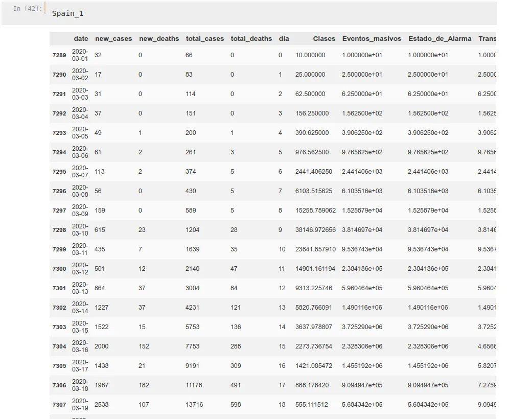
Spain_1 = Spain
Spain_1['dia'] = np.arange(0, len(Spain))
Spain_1['Clases'] = R0_1_Spain*np.hstack([np.full((len(Spain[Spain['date']<='2020-03-09'])), 1), np.full((len(Spain[Spain['date']>'2020-03-09'])), 0.25)]) 
Spain_1['Eventos_masivos'] = R0_1_Spain*np.hstack([np.full((len(Spain[Spain['date']<='2020-03-14'])), 1), np.full((len(Spain[Spain['date']>'2020-03-14'])), 0.25)]) 
Spain_1['Estado_de_Alarma'] = R0_1_Spain*np.hstack([np.full((len(Spain[Spain['date']<='2020-03-14'])), 1), np.full((len(Spain[Spain['date']>'2020-03-14'])), 0.25)]) 
Spain_1['Transporte_publico'] = R0_1_Spain*np.hstack([np.full((len(Spain[Spain['date']<='2020-03-14'])), 1), np.full((len(Spain[Spain['date']>'2020-03-14'])), 0.5)]) 
Spain_1['Ejercicio_en_publico'] = R0_1_Spain*np.hstack([np.full((len(Spain[Spain['date']<='2020-03-14'])), 1), np.full((len(Spain[Spain['date']>'2020-03-14'])), 0.25)]) 
Spain_1['Tiendas_abiertas_al_publico'] = R0_1_Spain*np.hstack([np.full((len(Spain[Spain['date']<='2020-03-14'])), 1), np.full((len(Spain[Spain['date']>'2020-03-14'])), 0.25)]) 
Spain_1['Medical_Quality'] = R0_1_Spain*np.hstack([np.full((len(Spain)), 0.25)])
Spain_1 = Spain_1.fillna(0)

Now, we have a (probably not very good!) approximation for propagation rates at each moment. We get a geometric function using those factors, storing them at numpy arrays, and then we substitute the data on the DataFrame:

Prop_1Clases = [10]
for i in np.arange(0, len(Spain_3)-1):
    Prop_1Clases.append(Prop_1Clases[-1]*Spain_1['Clases'][Spain_1.index[0]+i])
Prop_1Eventos = [10]
for i in np.arange(0, len(Spain_3)-1):
    Prop_1Eventos.append(Prop_1Eventos[-1]*Spain_1['Eventos_masivos'][Spain_1.index[0]+i] )
Prop_1Alarma = [10]
for i in np.arange(0, len(Spain_3)-1):
    Prop_1Alarma.append(Prop_1Alarma[-1]*Spain_1['Estado_de_Alarma'][Spain_1.index[0]+i])
Prop_1Transprte = [10]
for i in np.arange(0, len(Spain_3)-1):
    Prop_1Transprte.append(Prop_1Transprte[-1]*Spain_1['Transporte_publico'][Spain_1.index[0]+i])
Prop_1Ejercicio = [10]
for i in np.arange(0, len(Spain_3)-1):
    Prop_1Ejercicio.append(Prop_1Ejercicio[-1]*Spain_1['Ejercicio_en_publico'][Spain_1.index[0]+i])
Prop_1Tiendas = [10]
for i in np.arange(0, len(Spain_3)-1):
    Prop_1Tiendas.append(Prop_1Tiendas[-1]*Spain_1['Tiendas_abiertas_al_publico'][Spain_1.index[0]+i])
Prop_1Medical = [10]
for i in np.arange(0, len(Spain_3)-1):
    Prop_1Medical.append(Prop_1Medical[-1]*Spain_1['Medical_Quality'][Spain_1.index[0]+i])    
    
Spain_1.drop(['Clases', 'Eventos_masivos', 'Eventos_masivos', 'Estado_de_Alarma', 'Transporte_publico', 'Ejercicio_en_publico', 'Tiendas_abiertas_al_publico', 'Medical_Quality'], axis=1, inplace=True)            
Spain_1['Clases'] = Prop_1Clases
Spain_1['Eventos_masivos'] = Prop_1Eventos
Spain_1['Estado_de_Alarma'] = Prop_1Alarma
Spain_1['Transporte_publico'] = Prop_1Transprte
Spain_1['Ejercicio_en_publico'] = Prop_1Ejercicio
Spain_1['Tiendas_abiertas_al_publico'] = Prop_1Tiendas
Spain_1['Medical_Quality'] = Prop_1Medical

We do this for every propagation rate and for every country, getting dataframes similar to this one:

Now we have out dataframes per country ready, we stack them up. We aggregate propagation data on one hand and deaths data on the other one, stacking countries one on one. First, China, then Italy, Spain, and finally UK, which will be the one we will try to predict.

We stack these data two times, getting a retard of 20 days on one hand and a retard of 15 days on the other. The propagation data columns are ‘[6, 7, 8, 9, 10, 11, 12]’ and we vertically stack each country. Despite this piece of code may seem long it is just an iteration of the same code all the time.

Stack_1_1RO_1 = np.vstack([China_1.iloc[:-20, [6, 7, 8, 9, 10, 11, 12]].values/60, Italy_1.iloc[:-20, [6, 7, 8, 9, 10, 11, 12]].values/61])
Stack_1_1RO_2 = np.vstack([China_2.iloc[:-20, [6, 7, 8, 9, 10, 11, 12]].values/60, Italy_2.iloc[:-20, [6, 7, 8, 9, 10, 11, 12]].values/61])
Stack_1_1RO_3 = np.vstack([China_3.iloc[:-20, [6, 7, 8, 9, 10, 11, 12]].values/60, Italy_3.iloc[:-20, [6, 7, 8, 9, 10, 11, 12]].values/61])
Stack_1_2RO_1 =  Spain_1.iloc[:-20, [6, 7, 8, 9, 10, 11, 12]].values/47
Stack_1_2RO_2 =  Spain_2.iloc[:-20, [6, 7, 8, 9, 10, 11, 12]].values/47
Stack_1_2RO_3 =  Spain_3.iloc[:-20, [6, 7, 8, 9, 10, 11, 12]].values/47
Stack_1_3RO_1 = np.vstack((Stack_1_1RO_1,Stack_1_2RO_1))
Stack_1_3RO_2 = np.vstack((Stack_1_1RO_2,Stack_1_2RO_2))
Stack_1_3RO_3 = np.vstack((Stack_1_1RO_3,Stack_1_2RO_3))
Stack_1_4RO_1 =  UK_1.iloc[5:-15, [6, 7, 8, 9, 10, 11, 12]].values/67
Stack_1_4RO_2 =  UK_2.iloc[5:-15, [6, 7, 8, 9, 10, 11, 12]].values/67
Stack_1_4RO_3 =  UK_3.iloc[5:-15, [6, 7, 8, 9, 10, 11, 12]].values/67
Stack_1_5RO_1 = np.vstack((Stack_1_3RO_1,Stack_1_4RO_1))
Stack_1_5RO_2 = np.vstack((Stack_1_3RO_2,Stack_1_4RO_2))
Stack_1_5RO_3 = np.vstack((Stack_1_3RO_3,Stack_1_4RO_3))
Stack_2_1RO_1 = np.vstack([China_1.iloc[5:-15, [6, 7, 8, 9, 10, 11, 12]].values/60, Italy_1.iloc[5:-15, [6, 7, 8, 9, 10, 11, 12]].values/61])
Stack_2_1RO_2 = np.vstack([China_2.iloc[5:-15, [6, 7, 8, 9, 10, 11, 12]].values/60, Italy_2.iloc[5:-15, [6, 7, 8, 9, 10, 11, 12]].values/61])
Stack_2_1RO_3 = np.vstack([China_3.iloc[5:-15, [6, 7, 8, 9, 10, 11, 12]].values/60, Italy_3.iloc[5:-15, [6, 7, 8, 9, 10, 11, 12]].values/61])
Stack_2_2RO_1 =  Spain_1.iloc[5:-15, [6, 7, 8, 9, 10, 11, 12]].values/47
Stack_2_2RO_2 =  Spain_2.iloc[5:-15, [6, 7, 8, 9, 10, 11, 12]].values/47
Stack_2_2RO_3 =  Spain_3.iloc[5:-15, [6, 7, 8, 9, 10, 11, 12]].values/47
Stack_2_3RO_1 = np.vstack((Stack_2_1RO_1,Stack_2_2RO_1))
Stack_2_3RO_2 = np.vstack((Stack_2_1RO_2,Stack_2_2RO_2))
Stack_2_3RO_3 = np.vstack((Stack_2_1RO_3,Stack_2_2RO_3))
Stack_2_4RO_1 =  UK_1.iloc[10:-10, [6, 7, 8, 9, 10, 11, 12]].values/67
Stack_2_4RO_2 =  UK_2.iloc[10:-10, [6, 7, 8, 9, 10, 11, 12]].values/67
Stack_2_4RO_3 =  UK_3.iloc[10:-10, [6, 7, 8, 9, 10, 11, 12]].values/67
Stack_2_5RO_1 = np.vstack((Stack_2_3RO_1,Stack_2_4RO_1))
Stack_2_5RO_2 = np.vstack((Stack_2_3RO_2,Stack_2_4RO_2))
Stack_2_5RO_3 = np.vstack((Stack_2_3RO_3,Stack_2_4RO_3))
Prop1 = np.hstack((Stack_1_5RO_1, Stack_2_5RO_1))
Prop2 = np.hstack((Stack_1_5RO_2, Stack_2_5RO_2))
Prop3 = np.hstack((Stack_1_5RO_3, Stack_2_5RO_3))

Special attention to the fact we are dividing the propagation and death data by the millions of people each country has as population, so we have a propagation adjusted to each country. Despite China has a way bigger population, we are using 60 Million people as measure, since it is approximately the population of the Hubei province, main focus of the epidemy.

The deaths pass over the same process, only this time it is the column [4] (total_deaths) and the data is taken between 10 and 5 day before the prediction.

Stack_3_1RO_1 = np.vstack([China_1.iloc[10:-10, [4]].values/60, Italy_1.iloc[10:-10, [4]].values/61])
Stack_3_1RO_2 = np.vstack([China_2.iloc[10:-10, [4]].values/60, Italy_2.iloc[10:-10, [4]].values/61])
Stack_3_1RO_3 = np.vstack([China_3.iloc[10:-10, [4]].values/60, Italy_3.iloc[10:-10, [4]].values/61])
Stack_3_2RO_1 =  Spain_1.iloc[10:-10, [4]].values/47
Stack_3_2RO_2 =  Spain_2.iloc[10:-10, [4]].values/47
Stack_3_2RO_3 =  Spain_3.iloc[10:-10, [4]].values/47
Stack_3_3RO_1 = np.vstack((Stack_3_1RO_1,Stack_3_2RO_1))
Stack_3_3RO_2 = np.vstack((Stack_3_1RO_2,Stack_3_2RO_2))
Stack_3_3RO_3 = np.vstack((Stack_3_1RO_3,Stack_3_2RO_3))
Stack_3_4RO_1 =  UK_1.iloc[15:-5, [4]].values/67
Stack_3_4RO_2 =  UK_2.iloc[15:-5, [4]].values/67
Stack_3_4RO_3 =  UK_3.iloc[15:-5, [4]].values/67
Stack_3_5RO_1 = np.vstack((Stack_3_3RO_1,Stack_3_4RO_1))
Stack_3_5RO_2 = np.vstack((Stack_3_3RO_2,Stack_3_4RO_2))
Stack_3_5RO_3 = np.vstack((Stack_3_3RO_3,Stack_3_4RO_3))
Stack_4_1RO_1 = np.vstack([China_1.iloc[15:-5, [4]].values/60, Italy_1.iloc[15:-5, [4]].values/61])
Stack_4_1RO_2 = np.vstack([China_2.iloc[15:-5, [4]].values/60, Italy_2.iloc[15:-5, [4]].values/61])
Stack_4_1RO_3 = np.vstack([China_3.iloc[15:-5, [4]].values/60, Italy_3.iloc[15:-5, [4]].values/61])
Stack_4_2RO_1 =  Spain_1.iloc[15:-5, [4]].values/47
Stack_4_2RO_2 =  Spain_2.iloc[15:-5, [4]].values/47
Stack_4_2RO_3 =  Spain_3.iloc[15:-5, [4]].values/47
Stack_4_3RO_1 = np.vstack((Stack_4_1RO_1,Stack_4_2RO_1))
Stack_4_3RO_2 = np.vstack((Stack_4_1RO_2,Stack_4_2RO_2))
Stack_4_3RO_3 = np.vstack((Stack_4_1RO_3,Stack_4_2RO_3))
Stack_4_4RO_1 =  UK_1.iloc[20:, [4]].values/67
Stack_4_4RO_2 =  UK_2.iloc[20:, [4]].values/67
Stack_4_4RO_3 =  UK_3.iloc[20:, [4]].values/67
Stack_4_5RO_1 = np.vstack((Stack_4_3RO_1,Stack_4_4RO_1))
Stack_4_5RO_2 = np.vstack((Stack_4_3RO_2,Stack_4_4RO_2))
Stack_4_5RO_3 = np.vstack((Stack_4_3RO_3,Stack_4_4RO_3))
Cases1 = np.hstack((Stack_3_5RO_1, Stack_4_5RO_1))
Cases2 = np.hstack((Stack_3_5RO_2, Stack_4_5RO_2))
Cases3 = np.hstack((Stack_3_5RO_3, Stack_4_5RO_3))

Same method for days

Stack_5_1RO_1 = np.vstack([China_1.iloc[20:, [5]].values, Italy_1.iloc[20:, [5]].values])
Stack_5_1RO_2 = np.vstack([China_2.iloc[20:, [5]].values, Italy_2.iloc[20:, [5]].values])
Stack_5_1RO_3 = np.vstack([China_3.iloc[20:, [5]].values, Italy_3.iloc[20:, [5]].values])
Stack_5_2RO_1 = Spain_1.iloc[20:, [5]].values
Stack_5_2RO_2 = Spain_2.iloc[20:, [5]].values
Stack_5_2RO_3 = Spain_3.iloc[20:, [5]].values
Stack_5_3RO_1 = np.vstack((Stack_5_1RO_1,Stack_5_2RO_1))
Stack_5_3RO_2 = np.vstack((Stack_5_1RO_2,Stack_5_2RO_2))
Stack_5_3RO_3 = np.vstack((Stack_5_1RO_3,Stack_5_2RO_3))
Stack_5_4RO_1 = UK_1.iloc[20:, [5]].values
Stack_5_4RO_2 = UK_2.iloc[20:, [5]].values
Stack_5_4RO_3 = UK_3.iloc[20:, [5]].values
Days1 = np.vstack((Stack_5_3RO_1,Stack_5_4RO_1))
Days2 = np.vstack((Stack_5_3RO_2,Stack_5_4RO_2))
Days3 = np.vstack((Stack_5_3RO_3,Stack_5_4RO_3))

Our Y…

Stack_6_1RO_1 = np.vstack([China_1.iloc[20:, [2]].values/60, Italy_1.iloc[20:, [2]].values/61])
Stack_6_1RO_2 = np.vstack([China_2.iloc[20:, [2]].values/60, Italy_2.iloc[20:, [2]].values/61])
Stack_6_1RO_3 = np.vstack([China_3.iloc[20:, [2]].values/60, Italy_3.iloc[20:, [2]].values/61])
Stack_6_2RO_1 =  Spain_1.iloc[20:, [2]].values/47
Stack_6_2RO_2 =  Spain_2.iloc[20:, [2]].values/47
Stack_6_2RO_3 =  Spain_3.iloc[20:, [2]].values/47
Stack_6_3RO_1 = np.vstack((Stack_6_1RO_1,Stack_6_2RO_1))
Stack_6_3RO_2 = np.vstack((Stack_6_1RO_2,Stack_6_2RO_2))
Stack_6_3RO_3 = np.vstack((Stack_6_1RO_3,Stack_6_2RO_3))
Stack_6_4RO_1 =  UK_1.iloc[20:, [2]].values/67
Stack_6_4RO_2 =  UK_2.iloc[20:, [2]].values/67
Stack_6_4RO_3 =  UK_3.iloc[20:, [2]].values/67
Y1 = np.log10(np.vstack((Stack_6_3RO_1,Stack_6_4RO_1)))
Y2 = np.log10(np.vstack((Stack_6_3RO_2,Stack_6_4RO_2)))
Y3 = np.log10(np.vstack((Stack_6_3RO_3,Stack_6_4RO_3)))

Now, we have our 3 X factors and our Y, we stack them together and preprocess them. Propagation and deaths data grow way too fast, so we convert them to logarithmic scale uppon our stacking.

Stackeo1 = np.log10(np.hstack((Prop1, Cases1)))
Stackeo2 = np.log10(np.hstack((Prop2, Cases2)))
Stackeo2 = np.log10(np.hstack((Prop3, Cases3)))
x1 = np.hstack((Stackeo1, Days1))
x2 = np.hstack((Stackeo2, Days2))
x3 = np.hstack((Stackeo2, Days3))

Converting to logarithmic scale may produce infinites, we convert these -inf to 0 and then normalize all our X’

x1[x1 == -inf] = 0
x2[x2 == -inf] = 0
x3[x3 == -inf] = 0
Y1[Y1 == -inf] = 0
Y2[Y2 == -inf] = 0
Y3[Y3 == -inf] = 0
from sklearn.preprocessing import MinMaxScaler
min_max_scaler1 = MinMaxScaler()
X1 = min_max_scaler1.fit_transform(x1)
min_max_scaler2 = MinMaxScaler()
X2 = min_max_scaler2.fit_transform(x2)
min_max_scaler3 = MinMaxScaler()
X3 = min_max_scaler3.fit_transform(x3)
min_max_scaler4 = MinMaxScaler()
Y1 = min_max_scaler4.fit_transform(Y1)
min_max_scaler5 = MinMaxScaler()
Y2 = min_max_scaler5.fit_transform(Y2)
min_max_scaler6 = MinMaxScaler()
Y3 = min_max_scaler6.fit_transform(Y3)

Ok, this has been long, I know, but we are almost done preparing the data. Finally, we use an ExtraTreesRegressor along with a SelectFromModel to see which of all this data we have gatheres is more relevant to our Y, and transform our X to those shapes.

from sklearn.ensemble import ExtraTreesRegressor
from sklearn.feature_selection import SelectFromModel
RF = ExtraTreesRegressor()
RF.fit(X1, Y1)
featureselector1 = SelectFromModel(RF, prefit=True)
X1 = featureselector1.transform(X1)
RF = ExtraTreesRegressor()
RF.fit(X2, Y2)
featureselector2 = SelectFromModel(RF, prefit=True)
X2 = featureselector2.transform(X2)
RF = ExtraTreesRegressor()
RF.fit(X3, Y3)
featureselector3 = SelectFromModel(RF, prefit=True)
X3 = featureselector3.transform(X3)
Shape1 = X1.shape[1]
Shape2 = X2.shape[1]
Shape3 = X3.shape[1]

Since we are using an LSTM now, which is probably the strongest tool to make this kind of work, we need to get a tridimensional matrix, made this way:

• Time steps
• Features
• Factors

So, we reshape our X’s and divide our data into train and test to quantify the quality of the different models we will try.

X1_train = X1[:-10].reshape(len(X1)-10, 1, X1.shape[1])
X2_train = X2[:-10].reshape(len(X2)-10, 1, X2.shape[1])
X3_train = X3[:-10].reshape(len(X3)-10, 1, X3.shape[1])
X1_test = X1[-10:].reshape(10, 1, X1.shape[1])
X2_test = X2[-10:].reshape(10, 1, X2.shape[1])
X3_test = X3[-10:].reshape(10, 1, X3.shape[1])
Y1_train = Y1[:-10]
Y2_train = Y2[:-10]
Y3_train = Y3[:-10]
Y1_test = Y1[-10:]
Y2_test = Y2[-10:]
Y3_test = Y3[-10:]

The models will be composed of 5 layers, where 2 will be LSTM and 3 Dense, all using ‘REctified Linear Unit’ (RELU) activation functions and trying both RMSProp and Adamax optimizations.

modelLSTM01_1 = Sequential()
modelLSTM01_1.add(LSTM(40, return_sequences=True))
modelLSTM01_1.add(LSTM(200, activation='relu'))
modelLSTM01_1.add(Dense(40, activation='relu'))
modelLSTM01_1.add(Dense(10, activation='relu'))
modelLSTM01_1.add(Dense(1, activation='relu'))
modelLSTM01_1.compile(optimizer='Adamax', loss='mae', metrics = ['mae'])
modelLSTM01_1.fit(X1_train, Y1_train, epochs=50, batch_size=1, verbose=1)
LSTMPredicton01_1 = modelLSTM01_1.predict(X1_test)
score, mae = modelLSTM01_1.evaluate(X1_test, Y1_test)
score = sqrt(mean_squared_error(LSTMPredicton01_1, Y1_test))
print('Test score:', score)
print('Accuracy:', mae)

We value the accuray over the test phase and the training phase to select our model. We do this with 6 different models.

This would be basically all. Now we have selected our model, to make our prediction we simply change our X, selecting 5 more days on the UK (or other country) data, as we can see on our the next phases of the git, which I won’t include in this article so it does not get longer.

Our data will be normalized an logarithmic. We may invert these doing:

10**(mix_max_scaler1.inverse_transform(LSTMPredicton01_1))

Which would get us a death per Million stat.

Hope this article is understandable enough despite its length.